Contents
Simple Gradients based visualization。
基于梯度的方法,做了仨事:
- Class Model Visualisation,一个优化问题:最大化目标标签的score,反向传播优化input image;
- Image-Specific Class Saliency Visualisation:提出通过目标标签的score(softmax前)在input image上的梯度,得出saliency map的可视化方法;
- Relation to Deconvolutional Networks:说明其generalize了deconv的可视化方法。
Class Model Visualisation
有一个已经训练完成的模型,求解以下问题生成该类别的在该模型下的可视化图:
其中
Image-Specific Class Saliency Visualisation
在已有模型
作为可视化结果。
可以将此可视化结果看作为非线性模型的线性近似,即在线性模型
下,
将非线性模型
即对
类别特征图提取
对于灰度图,直接使用上述公式;若是三通道,则是使用
实验
代码大改自https://github.com/ivanmontero/visualize-saliency,基于keras。
首先写几个操作组成:
导入库:1
2
3
4import numpy as np
import tensorflow as tf
from keras import backend as K
from keras import activations
归一化:1
2
3
4def normalize(array):
arr_min = np.min(array)
arr_max = np.max(array)
return (array - arr_min) / (arr_max - arr_min + K.epsilon())
去除softmax层:1
2
3def linearize_activation(model):
model.layers[-1].activation = activations.linear
return model
计算score相对于input image的梯度:1
2
3
4
5
6
7
8
9
10
11
12
13
14
15
16def compute_gradient(model, output_index, input_image):
input_tensor = model.input
output_tensor = model.output
loss_fn = output_tensor[:, output_index]
grad_fn = K.gradients(loss_fn, input_tensor)[0]
compute_fn = K.function([input_tensor],
[loss_fn, grad_fn])
computed_values = compute_fn([input_image])
loss, grads = computed_values
print(loss, grads)
return grads
生成可视化图,有个trick是由于grads太小,所以用1去减一下,可视化效果更好:1
2
3
4
5
6
7
8
9def visualize_saliency(model, output_index, input_image, custom_objects=None):
model = linearize_activation(model, custom_objects)
grads = compute_gradient(model, output_index, input_image)
channel_idx = 1 if K.image_data_format() == 'channels_first' else -1
grads = np.maximum(0, grads)
grads = np.max(grads, axis=channel_idx)
grads = 1.0 - grads
return normalize(grads)[0]
main函数:1
2
3
4
5
6
7
8
9
10
11
12
13
14
15
16
17
18
19
20
21
22
23
24
25
26if __name__ == '__main__':
from keras.applications import vgg16
from keras.preprocessing.image import load_img
from keras.preprocessing.image import img_to_array
from keras.applications.imagenet_utils import decode_predictions
import matplotlib.pyplot as plt
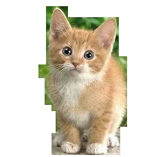
filename = 'cat2.jpg' #285
# 载入图像
original = load_img(filename, target_size=(224, 224))
numpy_image = img_to_array(original)
image_batch = np.expand_dims(numpy_image, axis=0)
processed_image = vgg16.preprocess_input(image_batch.copy())
# 正向传播(仅作演示)
vgg_model = vgg16.VGG16(weights='imagenet')
predictions = vgg_model.predict(processed_image)
label_vgg = decode_predictions(predictions)
print(label_vgg)
# 反向传播,生成saliency map
saliency_map = visualize_saliency(vgg_model, 285, processed_image)
plt.matshow(saliency_map, cmap='gray')
plt.savefig('cat_saliency_map.png')
plt.show()
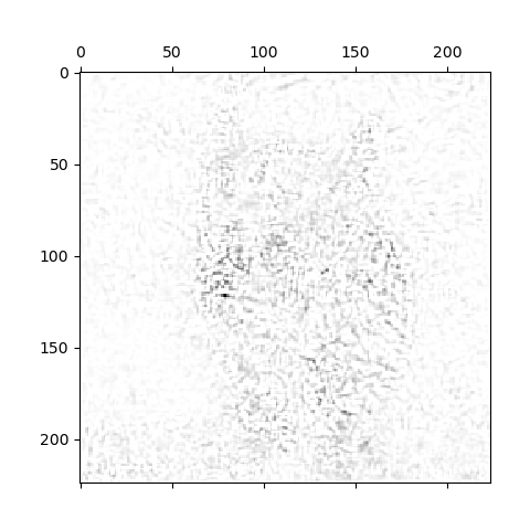
最后得到的效果如下:

Relation to Deconvolutional Networks
用
- 对于卷积层,第n的梯度为
即 ,即与deconv网络等价; - 对于ReLU层,反向传播时,第n层梯度
;而deconv网络为 。一个要求正向传播的特征大于零,另一则是梯度大于零。 - 对于池化层,由于deconv的switch的存在,所以等价。
然后作者说,除了ReLU,其余等价,且由于本文可以处理dense层,所以更general:
We can conclude that apart from the RELU layer, computing the approximate feature map reconstruction Rn using a DeconvNet is equivalent to computing the derivative ∂f /∂Xn using backpropagation, which is a part of our visualisation algorithms. Thus, gradient-based visualisation can be seen as the generalisation of that of [13], since the gradient-based techniques can be applied to the visualisation of activities in any layer, not just a convolutional one. In particular, in this paper we visualised the class score neurons in the final fully-connected layer.
笔记总结
对grad-cam中噪声的成因感兴趣,应该是由于背景信息中存在相似的pattern使得卷积核会提取到一点特征,如下面的显著图:
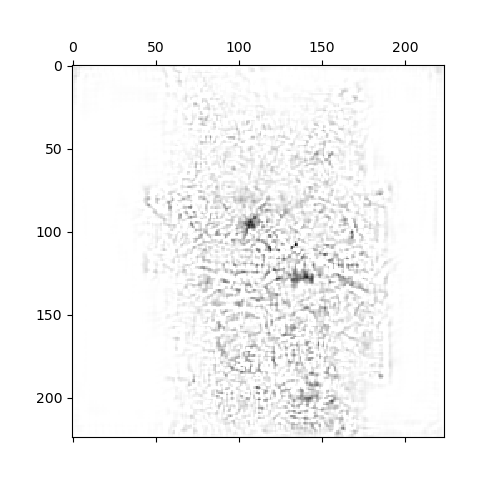
白色背景的显著图无噪声。