Note on understanding DFT

Contents

1. 1. Observation
2. 2. Understanding
   1. 2.0.1. DFT as Matrix-vector multiplication
   2. 2.0.2. Symmetries

I am going to give a quick explanation for DFT (Discrete Fourier Transform) from the viewpoint of DFT computation itself.

Observation

For example, here we use numpy.fft.fft for some random vectors:

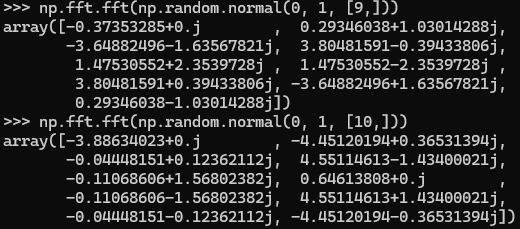
Let’s denote the input as , and the output as .

We can observe something about the result from fft:

• While most entries are complex numbers, the first entry is always a real number (i.e., the imaginary part is zero).
• Moreover, when the vector length is even, the is also a real number.
• and are conjugates of each other, for .

Understanding

DFT as Matrix-vector multiplication

Instead of telling a long story of DSP theory, let’s get an intuitive understanding directly from the computation process.

This is how fft computes from :

$$\begin{bmatrix} y_0\\ y_1\\ \vdots\\ y_{n-1} \end{bmatrix} = F\cdot \begin{bmatrix} x_0\\ x_1\\ \vdots\\ x_{n-1} \end{bmatrix}\\ \text{where}\;F=\begin{bmatrix} \omega^{0\times 0} & \omega^{1\times 0} & \omega^{2\times 0} & \cdots & \omega^{(n-1)\times 0} \\ \omega^{0\times 1} & \omega^{1\times 1} & \omega^{2\times 1} & \cdots & \omega^{(n-1)\times 1} \\ \vdots & \vdots & \vdots & \ddots & \vdots \\ \omega^{0\times (n-1)} & \omega^{1\times (n-1)} & \omega^{2\times (n-1)} & \cdots & \omega^{(n-1)\times (n-1)} \\ \end{bmatrix}\\ \omega^k=e^{-2\pi ik/n}$$

The matrix is called the Fourier matrix.

Essentially, ignoring the acceleration techniques, the fft can be viewed as a matrix-vector multiplication, where each is a weighted sum of the th row vector using the ‘weights’ .

$$y_s=\sum_t x_t\omega^{t\times s}=\sum_t x_t(e^{-2\pi si/n})^t$$

Let’s take a close look on these entries for a given row vector of matrix .

Symmetries

The th row vector of can be written as:

$$\begin{bmatrix}h_s(\frac{0}{n}) & h_s(\frac{1}{n}) & h_s(\frac{2}{n}) & \cdots & h_s(\frac{n-1}{n}) \\ \end{bmatrix}\;\text{where}\; h_s(x)=e^{-2\pi x\cdot si}$$

Therefore, this vector can be seen as sampling points in one period (i.e., ) of the periodic function .

In other words, the entries of th row vector is sampling points of frequency Hz. Respectively, the corresponding value is considered the Hz component of the original signal. For example, for the first row (=0), the frequency is zero and is simply the sum of . For the second row (), is of period and is input signal’s 1 Hz component.

Now let’s explain the above three observations by analyzing each row’s entries :

• For the first row, i.e., the frequency s=0,

  $$(e^{-2\pi si/n})^t=(e^{-2\pi ti/n})^s=(e^{-2\pi ti/n})^0=1$$

  So the first row vector’s entries are free of imaginary parts, is definitely a real number.

• Additionally, when n is even, for frequency

  $$(e^{-2\pi si/n})^t=(e^{-\pi i})^t=(e^{\pi i})^{-t}=(-1)^{-t}$$

  So these entries are also real numbers. Then, as a weighted sum of these entries, is definitely an real number.

• Moreover, we can observe that, for a th row’s entry:

  $$(e^{-2\pi (n-s)i/n})^t=(e^{2\pi si/n})^t=\overline{(\overline{e^{2\pi si/n}})^t}=\overline{(e^{-2\pi si/n})^t}$$

  It means the entries of th row vector and th row vector are conjugates of each other respectively. Therefore, and are also conjugates of each other, as they are linear combinations of these entries by the same weights.

  This implies that, given an input vector of entries, we can only obtain useful output values (see Nyquist sampling theorem). So, from the th output value, negative frequencies, i.e., Hz is used to call these output values. For example, given a vector length of 10, the output values are of frequencies 0 Hz, 1 Hz, 2 Hz, 3 Hz, 4 Hz, 5 Hz/-5 Hz, -4 Hz, -3Hz, -2 Hz, -1 Hz.

  So, after fft, if you want to shift the lower frequency components into the center, you use fftshift method to alter the output values’ positions into an order (-5 Hz) -4 Hz, -3 Hz, -2 Hz, -1 Hz, 0 Hz, 1 Hz, 2 Hz, 3Hz, 4 Hz, (5 Hz).

  

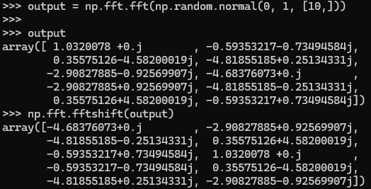
  Note that numpy.fft.fftshift regards the th output value as a part of negative frequencies.